Results
As for the experiments-overview, the results from the paper are divided in two categories: “Solution Quality” and “Running Time”.
Solution Quality
IP Formulation for MBI on Directed Graphs
The experiments clearly show that the experimental approximation ratio is by far better than the theoretical (see full paper [1] for prove). In fact, in all our tests, theexperimental ratio is always greater than \(0.96\).
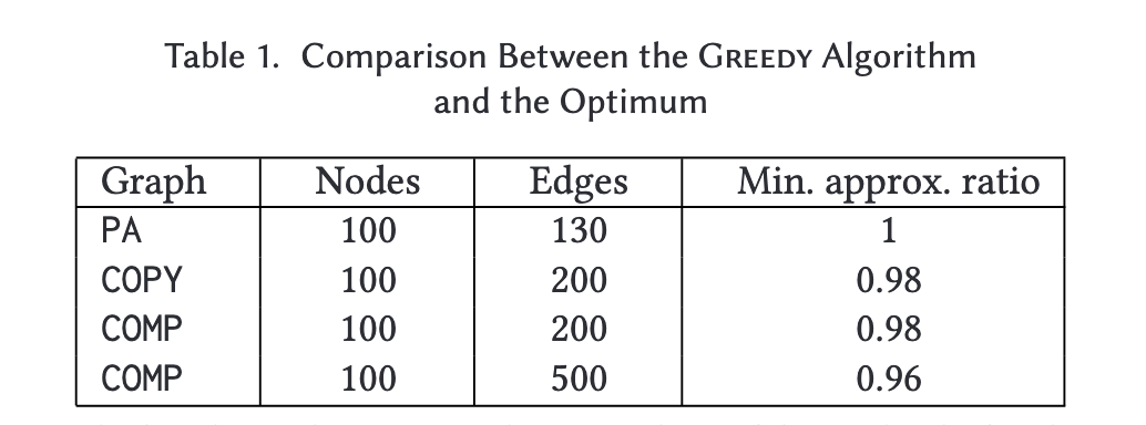
- Figure 1::
The first three columns report the type and size of the graphs; the fourthcolumn reports the approximation ratio.
Results for Real-World Directed Networks
Figure 2 shows the results for the munmun-digg-replygraph, using two different pivots. In particular, the plot on the left shows the betweenness improvement for a node with an initially low betweenness score (close to 0), whereas the one on the right refers to a node that starts with a higher betweenness value (about 40,000). Although the final betweenness scores reached by the two nodes differ, we see that the relative performance of the four algorithms is quite similar among the two pivots. A similar behavior can be observed for all other tested pivots and networks (see full paper [1] for all plots).
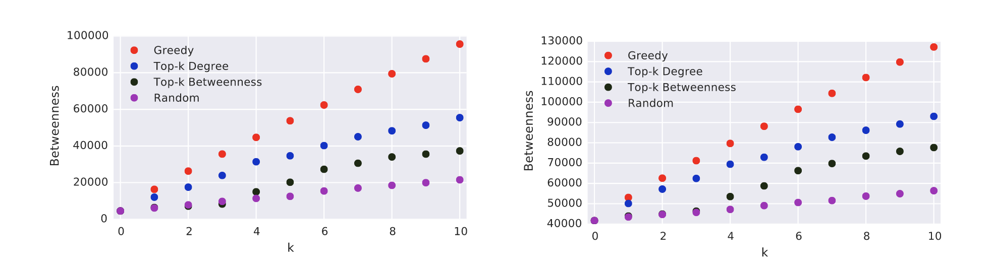
- Figure 2::
Betweenness of the pivot as a function of the numberkof inserted edges for the four heuristics. The plots refer to two different pivots in the munmun-digg-replygraph.
Figure 3 reports the average results over all directed networks, both in terms of betweenness (left) and rank (right) improvement. The initial average betweenness of the sample pivots is \(0.015%\). Greedy is by far the best approach, with an average final percentage betweenness (after 10 iterations) of \(0.38%\) and an average final percentage rank of \(1.4%\). As a comparison, the best alternative approach (Top-k Degree) yields a percentage betweenness of \(0.22%\) and a percentage rank of \(7.3%\). Not surprisingly, the worst approach is Random, which in 10 iterations yields afinal percentage betweenness of \(0.04%\) and an average percentage rank of \(10.2%\). On average, asingle iteration of Greedy is sufficient for a percentage rank of \(5.5%\), better than the one obtained by all other approaches in 10 iterations.
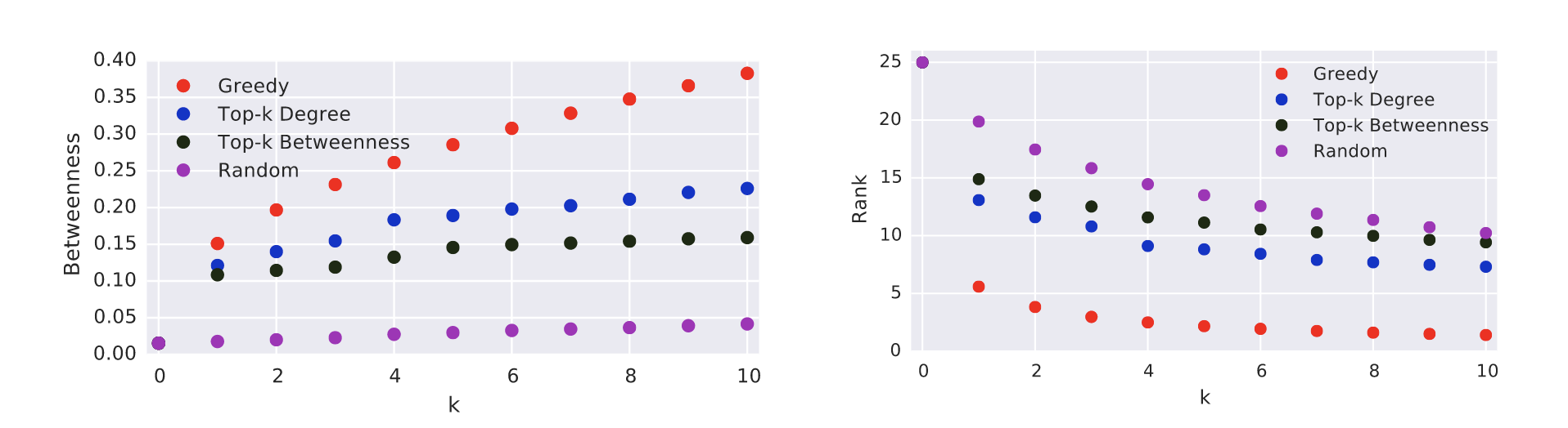
- Figure 3::
Average results over all directed networks. On the left, average percentage betweenness of the pivots as a function of k. On the right, average percentage rank of the pivots.
Results for Real-World Undirected Graphs
Figure 4 shows the percentage betweenness and ranking, averaged over the undirected networks. Also in this case, Greedy outperforms the other heuristics. In particular, the average initial betweenness of the pivots in the different graphs is \(0.05%\). After 10 iterations, the between-ness goes up to \(3.7%\) with Greedy, \(1.6%\) with Top-k Degree, \(2.1%\) with Top-k Betweenness and only \(0.17%\) with Random. The average initial rank is \(45%\). Greedy brings it down to \(0.7%\) with 10 iterations and below \(5%\) already with two. Using the other approaches, the average rank is always worse than \(10%\) for Top-k Betweenness, \(15%\) for Top-k Degree and \(20\) for Random. Differently from directed graphs, Top-k Betweenness performs significantly better than Top-k Degree in undirected graphs. Also, notice that in undirected graphs the percentage betweenness scores of the nodes in the examined graphs are significantly larger than those in the directed graphs. This could be due to the fact that many node pairs have an infinite distance in the examined directed graphs, meaning that these pairs do not contribute to the betweenness of any node. Also, say we want to increase thebetweenness of \(x\) by adding edge \((v,x)\). The pairs \((s,t)\) for which we can have a shortcut (leading to an increase in the betweenness of \(x\)) are limited to the ones such that scan reach \(v\) and such that \(t\) is reachable from \(x\), which might be a small fraction of the total number of pairs. On the contrary, most undirected graphs have a giant connected component containing the greatest majority of the nodes. Therefore, it is very likely that a pivot belongs to the giant component or that it will after the first edge insertion. It is interesting to notice that, despite the unbounded approximation ratio, the improvement achieved by Greedy on undirected graphs is even larger than for the directed ones: on average \(74\) times the initial score.
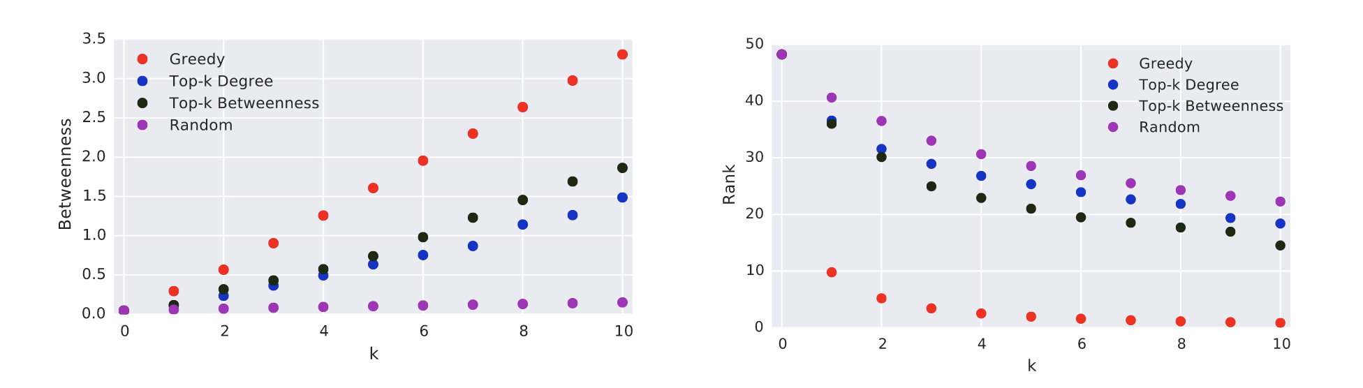
- Figure 4::
Average results over all undirected networks. On the left, average percentage betweenness of thepivots as a function ofk. On the right, average percentage rank of the pivots.
Running Time
Evaluation of the Dynamic Algorithm for the Betweenness of One Node
Figure 5 shows the speed up for directed and undirected graphs, respectively. As expected, both dynamic algorithms AI and SI are faster than the static approach and SI is the fastest among all algorithms. This is expected, since SI is the one that performs the smallest number of operations.
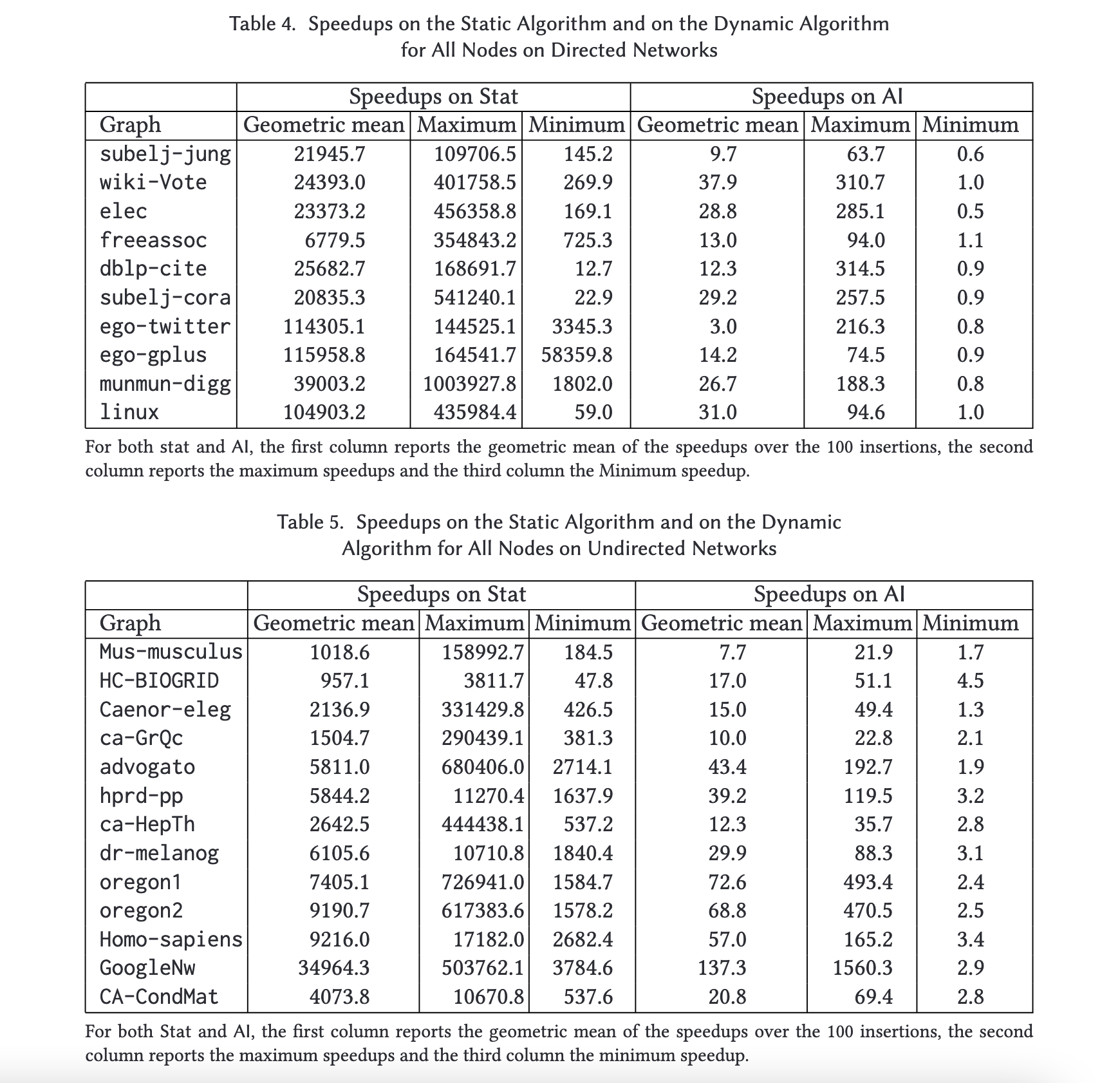
- Figure 5::
Speedups on the Static Algorithm and on the Dynamic Algorithm for All Nodes on Un/Directed Networks
Also, notice that the standard deviation of the running times of both AI and SI is very high, sometimes even higher than the average. This is actually not surprising, since different edge insertions might affect portions of the graph of very different sizes.
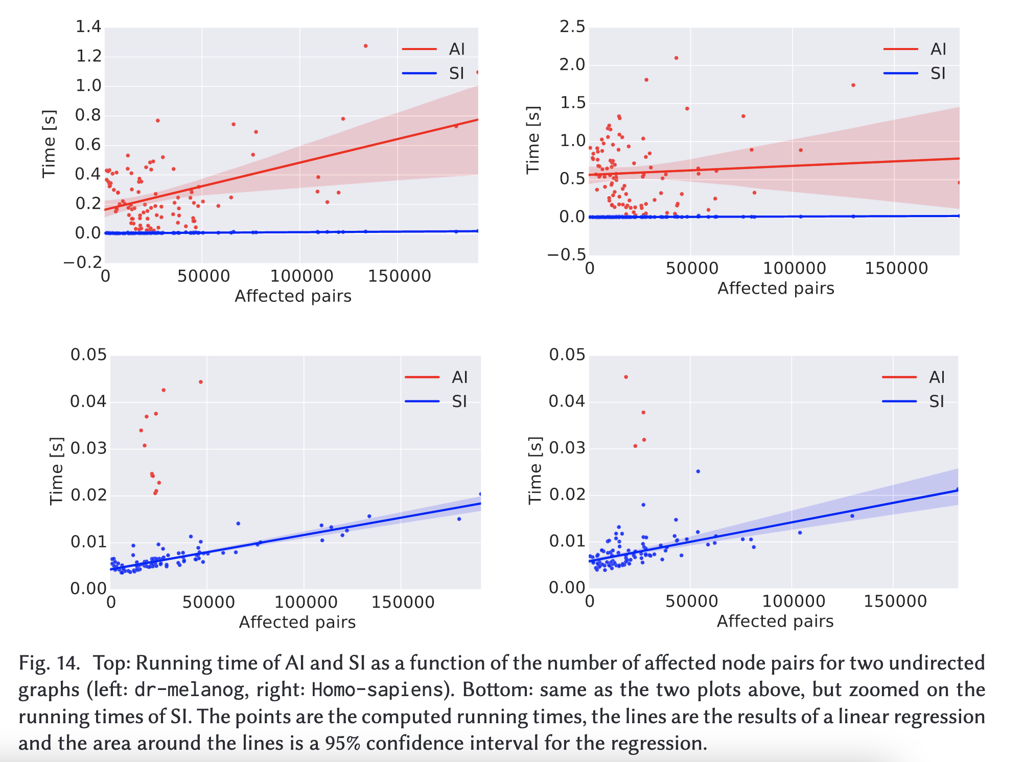
- Figure 6::
Speedups on the Static Algorithm and on the Dynamic Algorithm for All Nodes on Un/Directed Networks
Figure 6 reports the running times of AI and SI as a function of the number of affected node pairs for two directed and undirected graphs, respectively (similar results can be observed for the other tested graphs. As expected, the running time of both algorithms (as well as the difference between the running time of AI and that of SI) mostly increases as the number of affected pairs increases. However, AI presents a much larger deviation than SI. This is due to the fact that its running time also depends on the number of nodes that used to lie in old shortest paths between the affected pairs. Indeed,the number of nodes whose betweenness gets affected does not only depend on the number of affected pairs (which we recall to be the ones for which the edge insertion creates a shortcut or a
Running Times of the Greedy Algorithm for Betweenness Maximization
Figure 7 shows the results on directed andundirected graphs, respectively. For each value of \(k\), the figure shows the running time required by Greedy when \(k\) edges are added to the graph. Notice that this is not the running time of the \(kth\)-iteration, but the total running time of Greedy for a certain value of \(k\). Since on directed graphs the betweenness of \(x\) is a submodular function of the solutions for MBI, we can speed up the computation \(fork>1\). This technique was originally proposed in Reference [40] and it was used in Reference [16] to speed up the greedy algorithm for harmonic centrality maximization.
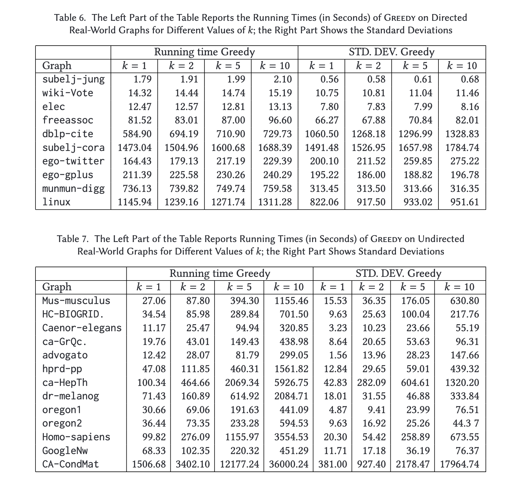
- Figure 7::
The Left Part Reports the Running Times (in Seconds) of Greedy on Un/Directed Real-World Graphs for Different Values of k; the Right Part Shows the Standard Deviations
Although the standard deviation is quite high, we can clearly see that exploiting submodularity has significant effects on the running times: for all graphs in Figure 7, we see that the difference in running time between computing the solution \(fork=1\) and \(k=10\) is at most a few seconds. Also,for all graphs the computation never takes more than a few minutes. Unfortunately, submodularity does not hold for undirected graphs, therefore for each \(k\) we needto apply SI to all possible new edges between \(x`and other nodes. Nevertheless, apart from the CA-CondMatgraph (where, on average, it takes about 10 hours :math:`fork=10\)) andca-HepTh (where it takes about \(1.5\) hours), Greedy never requires more than 1 hour \(fork=1\).