Experiments
We conduct experiments to demonstrate the performance of our approach compared to thestate-of-the-art competitors. Unless stated otherwise, we implemented all algorithms in C++, using the NetworKit [58] graph APIs. Our own algorithm is labelled \(UST\) in the results section. All experiments were conducted on a cluster with 16 Linux machines, each equippedwith an Intel Xeon 6126 CPU (2 sockets, 12 cores each), and 192 GB of RAM. To ensurere producibility, all experiments were managed by the SimexPal [5] software. For more technical details, have a look at our cluster overview page. We executed our experiments on the graphs in Tables below. All of them are unweighted and undirected. They have been downloaded from the public KONECT [35] repository and reduced to their largest connected component.
Quality Measures and Baseline
To evaluate the diagonal approximation quality, we measure the maximum absolute error (\(\max_i L^†_{ii} - \widetilde{L^†_{ii}}\)) on each instance, and we take both the maximum and the arithmetic mean over all the instances. Since for some applications [48] [49] a correct ranking of the entries is more relevant than their scores, in our experimental analysis we compare complete rankings of the elements of \(\widetilde{L^†}\). Note that the lowest entries of \(L^†\) (corresponding to the vertices with highest electrical closeness) are distributed on a significantly narrow interval. Hence, to achieve an accurate electrical closeness ranking ofthe topk vertices, one would need to solve the problem with very high accuracy. For this reason, all approximation algorithms we consider do not yield a precise top-kranking, so that we (mostly) consider the complete ranking. Using pinv in NumPy or Matlab as a baseline would be too expensive in terms of time (cubic) and space (quadratic) on large graphs. Thus, as quality baseline we employ the LAMG solver [40] as implemented within NetworKit [58] in our experiments (with \(10^{−9}\) tolerance). The results indicate that the diagonal obtained this way is sufficiently accurate.
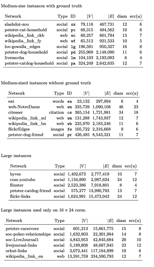
- Figure 1::
Real-world instance used for experiments. Image taken from full version of the paper [4]
Competitors in Practice
In practice, the fastest way to compute electrical closeness so faris to combine a dimension reduction via the Johnson-Lindenstrauss lemma [29] (JLT) with anumerical solver. In this context, Algebraic MultiGrid (AMG) solvers exhibit better empirical running time than fast Laplacian solvers with a worst-case guarantee [45]. For our experiments we use JLT combined with LAMG [40] (named Lamg-jlt); the latter is an AMG-type solverfor complex networks. We also compare against a Julia implementation of JLT together with the fast Laplacian solver proposed by Kyng et al. [36], for which a Julia implementation is already available in the package Laplacians.jl [f1]. This solver generates a sparse approximate Cholesky decomposition for Laplacian matrices with provable approximation guarantees in \(O(m\log^3{n}\log(1/\epsilon))\) time; it is based purely on random sampling (and does not make use of graph-theoretic concepts such as low-stretch spanning trees or sparsifiers). We refer to the above implementation as Julia-jlt throughout the experiments. For both Lamg-jlt and Julia-jlt,we try different input error bounds. This is a relative error, since these algorithms use numerical approaches with a relative error guarantee, instead of an absolute one (see Appendix E of the full version [4] for results in terms of different quality measures).
Finally, we compare against the diagonal estimators due to Bekas et al. [9], one based onrandom vectors and one based on Hadamard rows. To solve the resulting Laplacian systems, we use LAMG in both cases. In our experiments, the algorithms are referred to as Bekas and Bekas-h, respectively. Excluded competitors are discussed in Appendix D.1 (full version [4]).