Results
Running Time and Quality
For both Lamg-jlt and Julia-jlt, we try different input error bounds (they correspond to the respective numbers next to the method names in Figure 1). This is a relative error, since these algorithms use numerical approaches with a relative error guarantee, instead of an absolute one (see Appendix E of the full version [4] for results in terms of different quality measures).
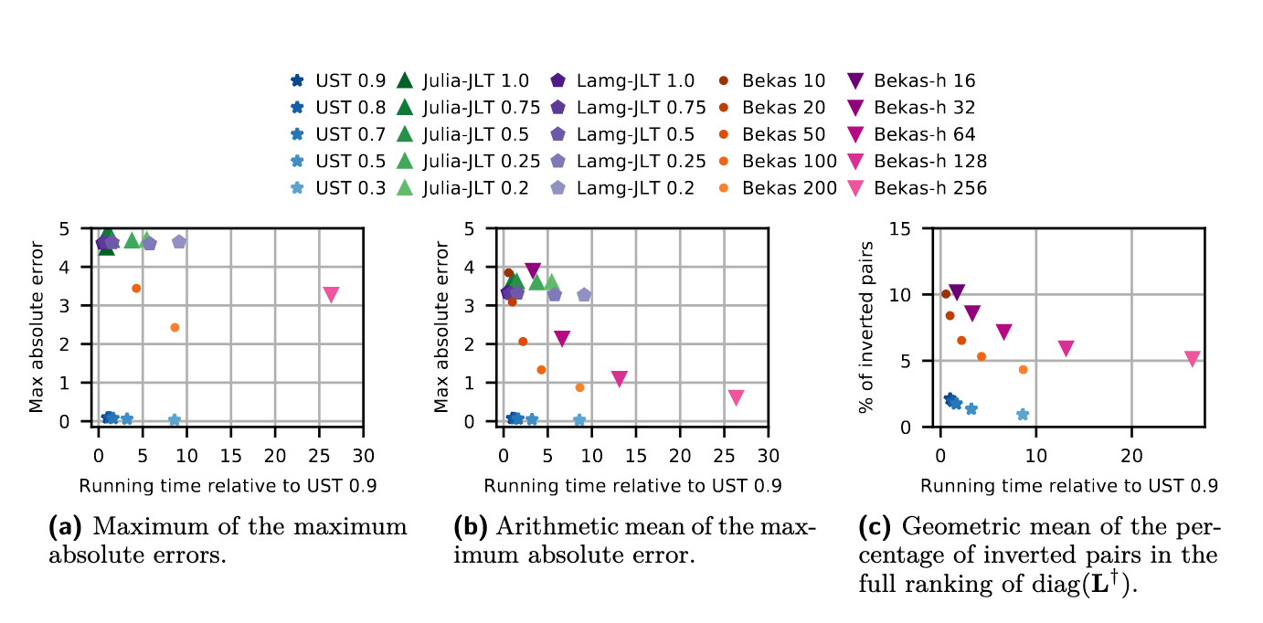
- Figure 1::
Quality results over the instances of Table 2 (full version [4]). All runs are sequential.
Figure 1a shows that, in terms of maximum absolute error, every configuration ofUSTachieves results with higher quality than the competitors. Even when setting \(\epsilon = 0.9\), UST yields a maximum absolute error of 0.09, and it is 8.3× faster than Bekas with 200 random vectors, which instead achieves a maximum absolute error of 2.43. Furthermore, the runningtime of UST does not increase substantially for lower values of \(\epsilon\), and its quality does not deteriorate quickly for higher values of \(\epsilon\). Regarding the average of the maximum absoluteerror, Figure 1b shows that, among the competitors,:code:Bekas-h with 256 Hadamard rows achieves the best precision. However, UST yields an average error of 0.07 while also being 25.4× faster than Bekas-h, which yields an average error of 0.62. Note also that the number next to each method in Figure 1 corresponds to different values of absolute (for UST) or relative (for Lamg-jlt, Julia-jlt) error bounds, and different numbers of samples (for Bekas, Bekas-h). For Bekas-h the number of samples needs to be a multiple of four due to the dimension of Hadamard matrices. In Figure 1c we report the percentage of inverted pairs in the full ranking of \(\widetilde{L^†}\). Note that JLT-based approaches are not depicted in this plot, because they yield >15% of rank inversions. Among the competitors, Bekas achieves the best time-accuracy trade-off. However, when using 200 random vectors, it yields 4.3% inversions while also being 8.3×slower than UST with \(\epsilon = 0.9\), which yields 2.1% inversions only.
Parallel Scalability
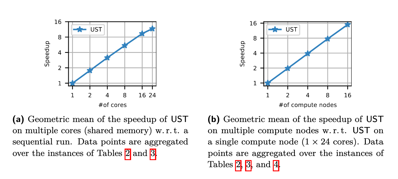
- Figure 2::
Scalability of
UST(\(\epsilon = 0.3\)) with shared and with distributed memory.
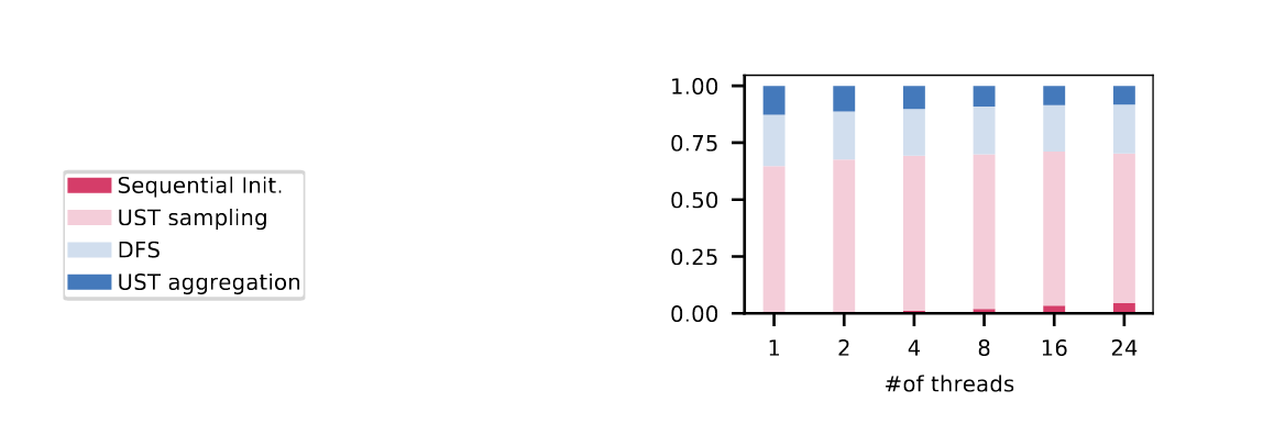
- Figure 3::
Breakdown of the running times of
USTwith \(\epsilon = 0.3\) w.r.t. #of cores on 1×24 cores. Data is aggregated with the geometric mean over the medium instances listed in the “Experiments” section.
The log-log plot in Figure 2a shows that on shared-memory UST achieves a moderate parallel scalability w.r.t. the number of cores; on 24 cores inparticular it is 11.9× faster than on a single core. Even though the number of USTs tobe sampled can be evenly divided among the available cores, we do not see a nearly-linear scalability: on multiple cores the memory performance of our NUMA system becomes a bottleneck. Therefore, the time to sample a UST increases and using more cores yields diminishing returns. Limited memory bandwidth is a known issue affecting algorithms based on graph traversals in general [7] [42]. Finally, we compare the parallel performance of UST indirectly with the parallel performance of our competitors. More precisely, assuming a perfect parallel scalability for our competitors Bekas and Bekas-h on 24 cores, UST would yield results 4.1 and 12.6 times faster, respectively, even with this strong assumption for the competition’s benefit. UST scales better in a distributed setting. In this case, the scalability is affected mainly by its non-parallel parts and by synchronization latencies. The log-log plot in Figure 2b shows that on up to 4 compute nodes the scalability is almost linear, while on 16 compute nodes UST achieves a 15.1× speedup w.r.t. a single compute node. Figure 3 shows the fraction of time that UST spends on different tasks depending on the number of cores. We aggregated over “Sequential Init.” the time spent on memory allocation, pivot selection, solving the linear system, the computation of the biconnected components, and on computing the tree \(B_u\). In all configurations, UST spends the majority of the time in sampling, computing the DFS data structures and aggregating USTs. The total time spent on aggregation corresponds to “UST aggregation”and “DFS” in Figure 3, indicating that computing the DFS data structures is the most expensive part of the aggregation. Together, sampling time and total aggregation timeaccount for 99.4% and 95.3% of the total running time on 1 core and 24 cores, respectively. On average, sampling takes 66.8% of this time, while total aggregation takes 31.2%. Since sampling a UST is on average 2.2× more expensive than computing the DFS timestamps and aggregation, faster sampling techniques would significantly improve the performance of our algorithm.
Scalability to Large Networks
Results on Synthetic Networks. The log-log plots in Figure 4a show the average running time of UST (1×24 cores) on networks generated with the random hyperbolic generator from von Looz et al. [61]. For each network size, we take the arithmetic mean of the running times measured for five different randomly generated networks. Our algorithm requires 184 minutes for the largest inputs (with up to 83.9 million edges). Interestingly, Figure 4b shows that the algorithm scales slightly better than our theoretical bound predicts. In Figure 6 (Appendix E.2, full version [4]) we present results on an additional graph class, namely R-MAT graphs. On these instances, the algorithm exhibits a similar running time behavior; however, the comparison to the theoretical bound is less conclusive.
Results on Large Real-World Networks. In Table 1 we report the performance of UST in a distributed setting (16×24cores) on large real-world networks. With \(\epsilon = 0.3\) and \(\epsilon = 0.9\), UST always runs in less than 8 minutes and 1.5 minutes, respectively.
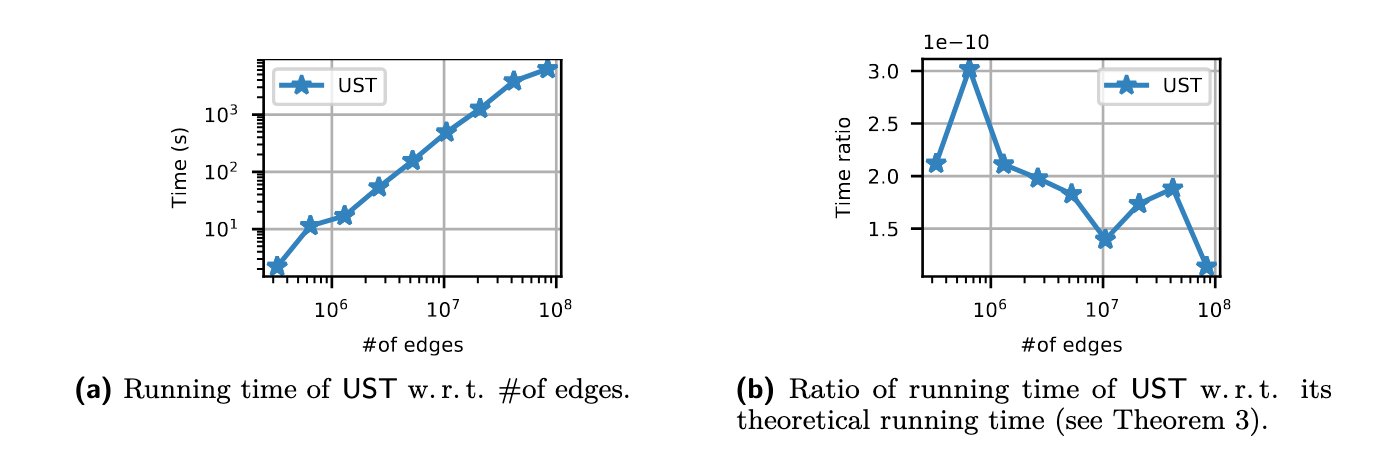
- Figure 4::
Scalability of
USTon random hyperbolic graphs (\(\epsilon = 0.3\), \(1 \times 24\) cores).